Pre-computation vs On-Demand Computation
Pre-computation trades storage and freshness for read speed by calculating results ahead of time.
Quick answer: Pre-computation vs On-Demand Computation
Pre-computation vs On-Demand Computation is covered here as a practical architecture tradeoff. Pre-computation trades storage and freshness for read speed by calculating results ahead of time. Use it when comparing two architecture choices and explaining the operational cost, latency, reliability, and team-complexity impact of each option.
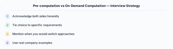
Focus on the problem being solved, the main design choice, the failure mode, and the tradeoff you would defend in front of a senior engineer. This page is part of the DosiBridge system design knowledge graph, so it links related concepts, interview problems, tradeoffs, and references instead of leaving the topic isolated.
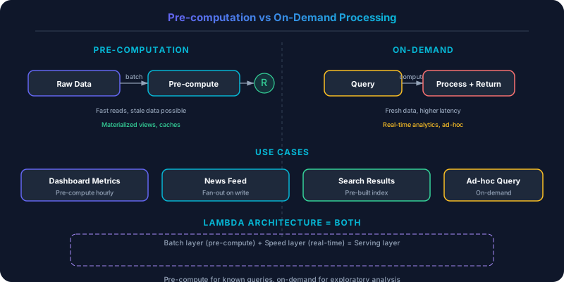
Pre-computation trades storage and freshness for read speed by calculating results ahead of time. On-demand computation trades latency for freshness and storage efficiency by calculating at query time. The choice shapes your system's performance profile.
Which Should You Pick?
Pre-compute if:
- The same computation is requested by many users (leaderboards, trending feeds)
- Read-to-write ratio is very high (1000:1 or more)
- Query latency requirements are strict (sub-10ms responses)
- The computation is expensive (aggregations over millions of rows)
Compute on-demand if:
- Results are unique per user or per request (search queries, personalized recommendations)
- Data changes frequently and staleness is unacceptable
- Storage is more expensive than compute for your use case
- The computation is cheap (single-row lookups, simple filters)
Understanding Pre-computation
Pre-computation calculates results before they are requested and stores them for instant retrieval. The computation happens during write time or in a background batch/stream process.
Strengths: Read latency is minimal — you are serving a pre-built result, not running a query. Database load during peak hours is low because the heavy computation happened offline. The system scales reads trivially by caching or replicating the pre-computed results.
Weaknesses: Storage costs increase because you are materializing results that might never be read. Freshness suffers — pre-computed results reflect the state at computation time, not query time. The pre-computation pipeline adds complexity: you must run it reliably, handle failures, and ensure results are consistent.
Twitter's home timeline is the textbook example. When you open Twitter, your home timeline is already pre-computed and waiting for you. When a user you follow posts a tweet, Twitter's fanout service writes that tweet ID to every follower's pre-computed timeline (stored in Redis). For a user with 1,000 followers, one tweet triggers 1,000 writes. The tradeoff: write amplification at post time in exchange for instant timeline reads. This works for most users, but for accounts with millions of followers (celebrities, news outlets), the fanout is too expensive. Twitter handles these with a hybrid approach: celebrity tweets are merged on-demand at read time.
YouTube's view counts are pre-aggregated. Real-time view counting for videos with millions of simultaneous viewers is computationally expensive. Instead, view events flow through Kafka into a stream processor that periodically writes aggregated counts to the database. The displayed count may lag behind the true count by seconds, but the read is a simple key lookup.
Understanding On-Demand Computation
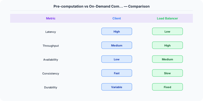
On-demand computation runs the calculation when the user requests it. The result is always fresh because it is derived from the current state of the data.
Strengths: Results are always current. No stale data, no consistency lag. Storage is minimal — you do not materialize results that nobody asks for. The system is simpler: no background pipelines, no pre-computation jobs, no materialized view maintenance.
Weaknesses: Read latency includes the full computation time. If the computation requires scanning millions of rows or joining multiple tables, the user waits. Database load is proportional to read traffic — every reader triggers computation. Under high concurrency, the database may become the bottleneck.
Google Search computes results on demand. Every search query is unique (or nearly so), which makes pre-computation impractical. Google cannot pre-compute results for every possible query. Instead, they invest heavily in making on-demand computation fast: inverted indexes, PageRank pre-computation (the ranking scores are pre-computed, but the query matching is on-demand), distributed query execution across thousands of servers, and aggressive caching of popular queries.
Stripe's dashboard analytics compute financial reports on demand. When a merchant views their revenue for a date range, the system queries the transaction database in real time. Pre-computing every possible date range for every merchant would require enormous storage. The tradeoff: reports for large merchants with millions of transactions take a few seconds to load.
Hybrid Approaches
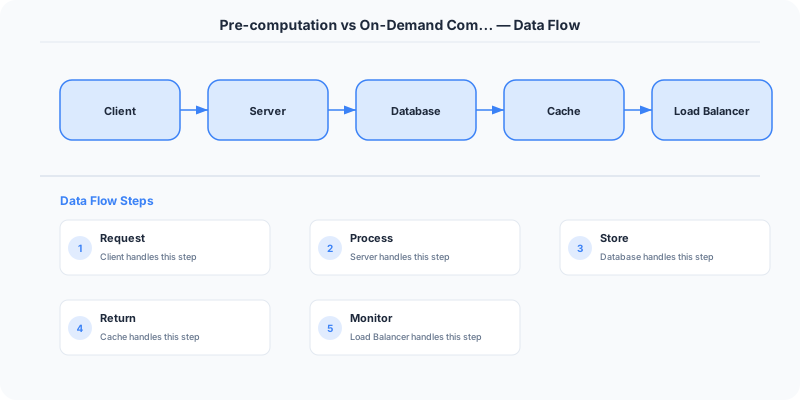
Most production systems blend both strategies:
Materialized views with incremental updates. Pre-compute a result set and update it incrementally as new data arrives. PostgreSQL's materialized views, Apache Flink's continuous queries, and DynamoDB Streams with Lambda all support this pattern. You get near-real-time freshness with read-time performance close to full pre-computation.
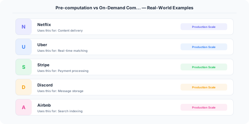
Pre-compute the common, compute the rare. Pre-compute results for the top 1% of queries that account for 80% of traffic. Compute everything else on demand. Netflix pre-computes recommendations for active users and generates them on demand for infrequent visitors.
Cache recent on-demand results. Compute on demand, cache the result with a TTL, and serve subsequent identical requests from cache. This gives you freshness on first access and speed for repeated access. Elasticsearch queries at LinkedIn follow this pattern: the first search is computed against the index, and the result is cached for subsequent identical searches.
Cost Analysis
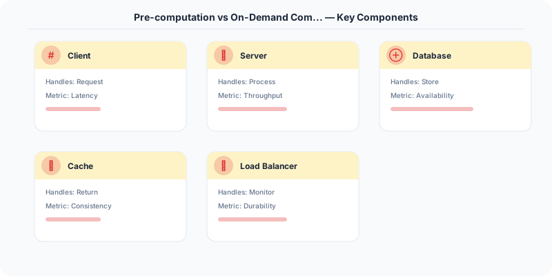
The economic tradeoff depends on your read-to-write ratio and computation cost:
Pre-computation cost = (number of possible results) x (storage cost per result) + (computation pipeline cost)
On-demand cost = (number of read requests) x (computation cost per request)
If you have 1 million users and each needs a personalized feed, pre-computing all feeds costs 1 million x computation time. If only 100,000 users log in daily, 90% of the pre-computation is wasted. On-demand computation for those 100,000 active users is cheaper.
Conversely, if you have a leaderboard that 10 million users view per hour but it only changes when scores update (a few thousand times per hour), pre-computing it once and serving 10 million reads from cache is vastly cheaper than running 10 million aggregation queries.
Side-by-Side Comparison
| Dimension | Pre-computation | On-Demand |
|---|---|---|
| Read Latency | Minimal (lookup) | Proportional to computation |
| Data Freshness | Potentially stale | Always current |
| Storage Cost | Higher (materialized results) | Lower |
| Write Amplification | Higher (fanout on write) | None |
| Complexity | Background pipelines | Simpler architecture |
| Best For | Hot, shared, expensive reads | Unique, cheap, or rare queries |
The rule of thumb: pre-compute when many readers consume the same expensive computation. Compute on demand when queries are unique or data freshness is paramount. Most systems land somewhere in between, with materialized views and caching bridging the gap.
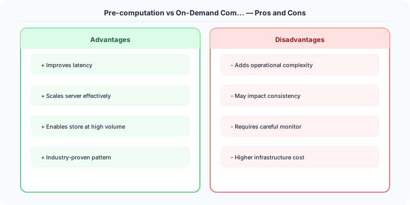
Original DosiBridge notes for Pre-computation vs On-Demand Computation
This section is written specifically for this page, not copied from a general system-design checklist. The useful way to study Pre-computation vs On-Demand Computation is to connect the concept to a production service where growth exposes the first weak assumption in the original design. That framing changes the design discussion from definitions to operating choices.
What makes this topic distinct
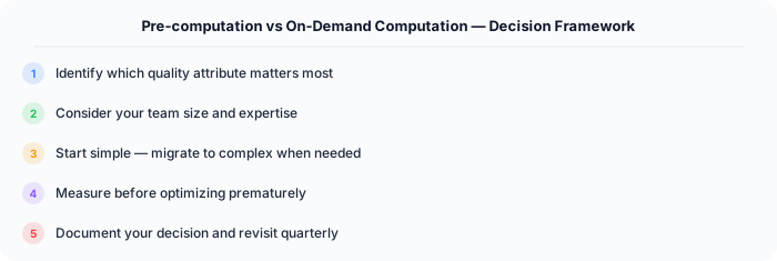
- Decision Boundary: For Pre-computation vs On-Demand Computation, decide the decision boundary before choosing tools; otherwise the design looks clean but fails when pre changes.
- Reversal Cost: For Pre-computation vs On-Demand Computation, decide the reversal cost before choosing tools; otherwise the design looks clean but fails when computation changes.
- Operating Cost: For Pre-computation vs On-Demand Computation, decide the operating cost before choosing tools; otherwise the design looks clean but fails when vs changes.
- Team Maturity: For Pre-computation vs On-Demand Computation, decide the team maturity before choosing tools; otherwise the design looks clean but fails when on changes.
- Growth Trigger: For Pre-computation vs On-Demand Computation, decide the growth trigger before choosing tools; otherwise the design looks clean but fails when demand changes.
Production review question
If a team adopts Pre-computation vs On-Demand Computation, what observable signal proves it helped instead of only making the architecture diagram more fashionable?
Practical metric to track
Track pre-demand health as a named dashboard or review item: combine one user-facing metric, one saturation metric, and one correctness metric. For Pre-computation vs On-Demand Computation, this keeps the discussion grounded in behavior that can be measured after deployment instead of generic advice that sounds good in an interview but never gets verified.