Rate Limiting Algorithms Explained
Quick answer: Rate Limiting Algorithms Explained
Rate Limiting Algorithms Explained is covered here as a practical system design article. A comparison of the four major rate limiting algorithms — token bucket, leaky bucket, fixed window, and sliding window — with tradeoffs and implementation. Use it to turn a broad system design idea into an interview-ready checklist with practical examples and links to deeper topics.
Focus on the problem being solved, the main design choice, the failure mode, and the tradeoff you would defend in front of a senior engineer. This page is part of the DosiBridge system design knowledge graph, so it links related concepts, interview problems, tradeoffs, and references instead of leaving the topic isolated.
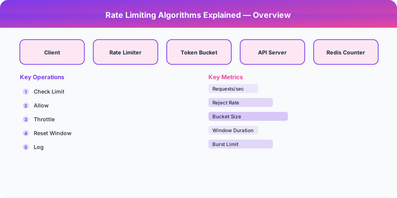
Rate Limiting Algorithms Explained
Rate limiting controls how many requests a client can make in a given time period. It protects servers from overload, ensures fair usage, and prevents abuse. The choice of algorithm determines how strictly the limit is enforced, how burst-friendly the system is, and how much memory is required.
Algorithm 1: Token Bucket
A bucket holds tokens, up to a maximum capacity. Each request consumes one token. Tokens are added to the bucket at a fixed rate (e.g., 10 tokens per second). If the bucket is empty, the request is rejected.
How it works: Initialize the bucket with a capacity of N tokens. On each request, check if tokens are available. If yes, decrement and allow. If no, reject. Refill tokens at the configured rate.
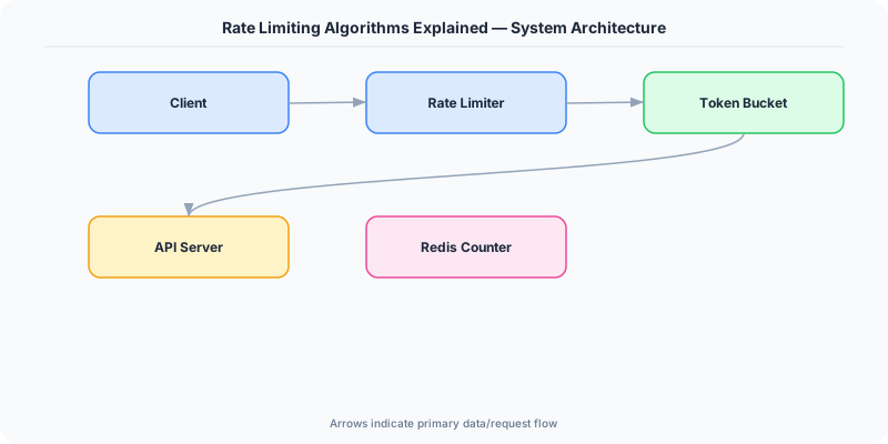
Implementation detail: You do not need a background thread to add tokens. Calculate the elapsed time since the last request and add the appropriate number of tokens (up to the capacity) at request time. This is called "lazy refill."
Behavior: Allows bursts up to the bucket capacity, then enforces the steady-state rate. A bucket with capacity 100 and rate 10/sec allows a burst of 100 requests, then 10/sec thereafter.
Pros: Simple, memory efficient (one counter + one timestamp per client), allows controlled bursts. Cons: Burst size is fixed by bucket capacity; tuning capacity and rate independently can be confusing.
Used by: AWS API Gateway, Stripe, many CDNs.
Algorithm 2: Leaky Bucket
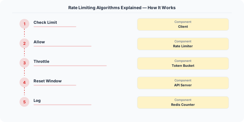
Requests enter a queue (the "bucket") and are processed at a fixed rate. If the queue is full, new requests are rejected.
How it works: Maintain a FIFO queue with a fixed capacity. Requests are added to the queue on arrival. A processor dequeues and processes requests at a constant rate.
Behavior: Smooths out bursts — even if 100 requests arrive at once, they are processed at the fixed rate. The queue absorbs bursts, but if the burst exceeds the queue capacity, excess requests are dropped.
Pros: Produces a perfectly smooth output rate, useful when downstream systems cannot handle bursts. Cons: Does not allow legitimate bursts (a user who has been idle should be able to make a few fast requests). Requires a queue data structure.
Used by: Network traffic shaping, some API gateways.
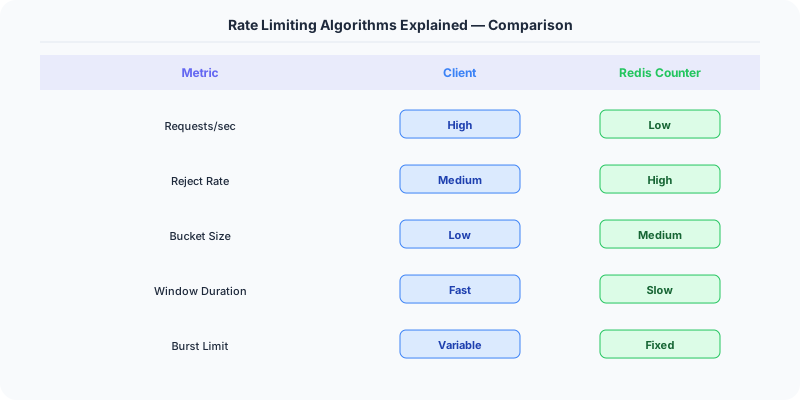
Algorithm 3: Fixed Window Counter
Divide time into fixed windows (e.g., each minute). Maintain a counter per window per client. If the counter exceeds the limit within the current window, reject the request.
How it works: Key = client_id + window_start_time. Increment the counter on each request. If counter > limit, reject.
Behavior: Simple to implement and memory-efficient. However, it has a boundary problem: a client can make the maximum requests at the end of one window and the beginning of the next, effectively doubling their rate for a brief period.
Example: Limit is 100 requests per minute. Client makes 100 requests at 11:00:59, then 100 more at 11:01:00. That is 200 requests in 2 seconds, despite a "100 per minute" limit.
Pros: Very simple, uses minimal memory (one counter per client per window). Cons: Boundary burst problem allows up to 2x the intended rate at window edges.
Algorithm 4: Sliding Window Log
Record the timestamp of every request in a sorted set. On each new request, remove timestamps older than the window and count the remaining entries. If the count exceeds the limit, reject.
How it works: Store timestamps in a sorted set (e.g., Redis ZSET). On request: remove entries older than (now - window_size), count remaining, allow if count < limit, add current timestamp.
Behavior: Perfectly accurate — no boundary burst problem. The window slides with each request.
Pros: Precise rate limiting with no edge cases. Cons: Memory-expensive — stores one timestamp per request per client. For a limit of 10,000 requests per hour, that is 10,000 entries per client.
Algorithm 5: Sliding Window Counter (Hybrid)
Combine fixed window and sliding window. Maintain counters for the current and previous windows. Estimate the rate by weighting the previous window's count based on how far into the current window we are.
How it works: Count for current window + (count for previous window * overlap percentage). If this weighted sum exceeds the limit, reject.
Example: Limit is 100/min. Previous window had 80 requests. Current window (30 seconds in) has 40 requests. Estimated count = 40 + 80 * 0.5 = 80. Under the limit, so allow.
Pros: Nearly as accurate as sliding window log, but uses only two counters per client (same as fixed window). Cons: An approximation — not perfectly precise, but good enough for almost all use cases.
Comparison Table
| Algorithm | Memory | Accuracy | Burst Handling | Complexity |
|---|---|---|---|---|
| Token Bucket | Low | Good | Allows controlled bursts | Low |
| Leaky Bucket | Medium | Good | Smooths all bursts | Medium |
| Fixed Window | Low | Poor (boundary issue) | Allows 2x burst at edges | Very low |
| Sliding Window Log | High | Perfect | No bursts beyond limit | Medium |
| Sliding Window Counter | Low | Good (approximate) | Minimal boundary issue | Low |
Which One Should You Use?
- Default choice: Token bucket. Simple, allows reasonable bursts, low memory.
- Smooth output needed: Leaky bucket. When downstream cannot handle any bursts.
- Memory-constrained, low accuracy OK: Fixed window. Simplest implementation.
- Precision critical: Sliding window log. When you cannot tolerate any over-limit requests.
- Best overall tradeoff: Sliding window counter. Near-perfect accuracy with minimal memory.
Original DosiBridge notes for Rate Limiting Algorithms Explained
This section is written specifically for this page, not copied from a general system-design checklist. The useful way to study Rate Limiting Algorithms Explained is to connect the concept to a traffic-management problem where overload behavior matters more than the happy-path diagram. That framing changes the design discussion from definitions to operating choices.
What makes this topic distinct
- Practical Lesson: For Rate Limiting Algorithms Explained, decide the practical lesson before choosing tools; otherwise the design looks clean but fails when rate changes.
- Migration Story: For Rate Limiting Algorithms Explained, decide the migration story before choosing tools; otherwise the design looks clean but fails when limiting changes.
- Production Symptom: For Rate Limiting Algorithms Explained, decide the production symptom before choosing tools; otherwise the design looks clean but fails when algorithms changes.
- Decision Checklist: For Rate Limiting Algorithms Explained, decide the decision checklist before choosing tools; otherwise the design looks clean but fails when explained changes.
- Rollback Plan: For Rate Limiting Algorithms Explained, decide the rollback plan before choosing tools; otherwise the design looks clean but fails when rate changes.
Production review question
If a team adopts Rate Limiting Algorithms Explained, what observable signal proves it helped instead of only making the architecture diagram more fashionable?
Practical metric to track
Track rate-explained health as a named dashboard or review item: combine one user-facing metric, one saturation metric, and one correctness metric. For Rate Limiting Algorithms Explained, this keeps the discussion grounded in behavior that can be measured after deployment instead of generic advice that sounds good in an interview but never gets verified.